Inverse matrices

Lecture 7

Minjae Park

Auburn University
MATH 2660 - Spring 2026

January 23, 2026

Announcement

  • HW 2 is due tonight at 11:59 PM.
  • On WebAssign, you can find Quiz 1 preparation, which includes all answers for review. Feel free to use it while studying for Quiz 1 or working on similar questions in HW 2.
  • As scheduled, Quiz 1 will take place during class next Friday (1/30/2026).

Attendance

Scan the QR code or go to join.iclicker.com/MBNJ.

Recap

Solving linear equations

  • A linear equation has the form \(A\vec{x}=\vec{b}\), where \(A\) is an \(n\times m\) matrix, \(\vec{x}\in\mathbb{R}^m\) is the vector of unknowns, and \(\vec{b}\in\mathbb{R}^n\) is the given vector.
  • The corresponding augmented matrix is written as \([A\mid\vec{b}]\).
  • To solve a system of linear equations, we apply Gauss–Jordan elimination to the augmented matrix using elementary row operations to obtain the reduced row-echelon form (RREF).
  • Depending on the final RREF, the system may have a unique solution, infinitely many solutions, or no solution.

Example 1

Consider the system of linear equations \[ \left\{\begin{aligned} x+2y+3z &= 9\\ 2x-y+z &= 8\\ 3x-z &= 3 \end{aligned}\right. \]

  • Write the associated augmented matrix.
  • Reduce it to reduced row-echelon form using Gauss–Jordan elimination.
  • Solve the system.
  • How many solutions are there?
    (Submit your answer to iClicker.)

Scan the QR code or go to join.iclicker.com/MBNJ.

Note: If you are completely lost or encounter difficulties, briefly explain your situation instead.

Example 2

Consider the augmented matrix \[ \left[\begin{array}{ccc|c} 1 & 3 & 1 & 0\\ 0 & 0 & 1 & 2\\ 0 & 0 & 0 & 0 \end{array}\right]. \]

  • Is this matrix in reduced row-echelon form? If not, reduce it.
  • Let the variables be \(x,y,z\). Solve the corresponding system.
  • How many solutions are there?
    (Submit your answer to iClicker.)

Scan the QR code or go to join.iclicker.com/MBNJ.

Note: If you are completely lost or encounter difficulties, briefly explain your situation instead.

Inverse matrices

Review: linear transformations on \(\mathbb{R}^2\)

  • Recall that a linear transformation \(A:\mathbb{R}^2\to\mathbb{R}^2\) describes how points in the plane are deformed linearly.
  • If \(\vec{v}_1=A\vec{e}_1\) and \(\vec{v}_2=A\vec{e}_2\), then a vector \[\vec{x}=\langle x_1,x_2 \rangle=x_1\vec{e}_1+x_2\vec{e}_2\] is mapped to \[\vec{y}=A\vec{x}=x_1\vec{v}_1+x_2\vec{v}_2.\]
  • Geometrically, \(A\) is completely determined by how the unit square spanned by \(\vec{e}_1,\vec{e}_2\) is transformed into the parallelogram spanned by \(\vec{v}_1,\vec{v}_2\).

Visualizing linear transformations

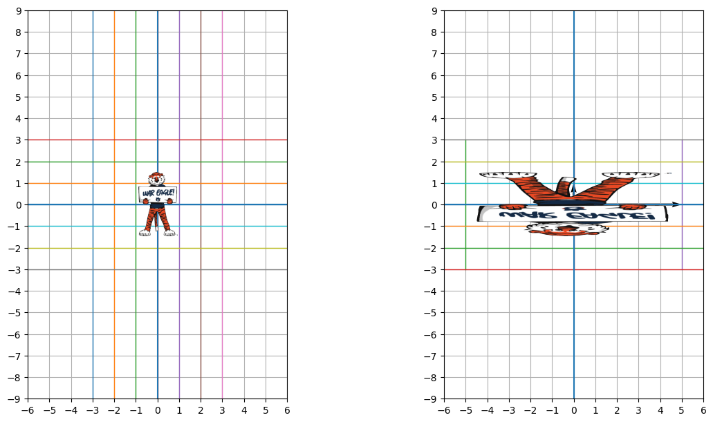
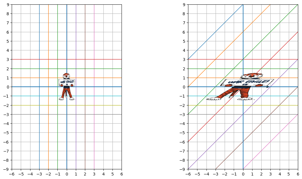
  • Each coordinate vector defines an axis, and together they generate a grid on the plane.
  • The deformed picture can be understood by tracking how this grid changes. For example, Aubie’s head is located at \((0,1)\) in every coordinate system.
Undo a linear transformation

  • Since a linear transformation is determined by how it transforms the grid of unit squares, we may ask whether there exists a linear transformation \[B:\mathbb{R}^2\to\mathbb{R}^2\] that maps the parallelogram spanned by \(\vec{v}_1,\vec{v}_2\) back to the unit square spanned by \(\vec{e}_1,\vec{e}_2\).
  • Such a transformation \(B\) would undo the effect of \(A\), and vice versa.
  • In other words, for any vector \(\vec{x}, \vec{y}\in \mathbb{R}^2\), \[\vec{x}=B(A(\vec{x})) = B\circ A (\vec{x}),\] \[\vec{y}=A(B(\vec{y})) = A\circ B (\vec{y}).\]

Matrix multiplication as composition

  • Consider two linear transformations \(A,B:\mathbb{R}^n\to\mathbb{R}^n\).
  • They are represented by matrices \[A=[\vec{a}_1\ \vec{a}_2\ \dots \ \vec{a}_n],\qquad B=[\vec{b}_1\ \vec{b}_2\ \dots \ \vec{b}_n].\]
  • Fact: the composition \(C = A\circ B\), read as “apply \(B\) first, then apply \(A\)”, is also a linear transformation.
  • How can we represent the matrix of the linear transformation \(C\)?

Matrix multiplication as composition

  • The matrix \(C = [\vec{c}_1\ \vec{c}_2\ \dots \ \vec{c}_n]\) is determined by how it acts on the coordinate vectors \(\vec{e}_i\).
  • Observe that \[\vec{c}_i = C\vec{e}_i = A(B\vec{e}_i)=A \vec{b}_i.\]
  • This is exactly how we defined the matrix multiplication \(AB\).
  • Hence, the matrix representing \(A\circ B\) is the matrix product \(AB\).
  • Similarly, the composition \(B\circ A\) is represented by the matrix \(BA\).

Inverse matrix

  • Let \(A:\mathbb{R}^n \to \mathbb{R}^n\) be a linear transformation.
  • If another linear transformation \(B:\mathbb{R}^n \to \mathbb{R}^n\) undoes what \(A\) does (and vice versa), then \[AB=BA=I_n,\] where \(I_n\) is the \(n \times n\) identity matrix.
  • Fact: if such a matrix \(B\) exists, it is unique, and \(A\) is called invertible.
  • This matrix \(B\) is called the inverse matrix of \(A\), denoted by \(A^{-1}\).

Relation to linear equations

  • Suppose we want to solve the linear equation \[A\vec{x}=\vec{b}.\]
  • If \(A\) has an inverse matrix, we can “undo” \(A\) by multiplying both sides by \(A^{-1}\): \[\vec{x}=A^{-1}A\vec{x}=A^{-1}\vec{b}.\]
  • This produces a single vector solution, so the solution is unique.
  • Therefore, a matrix \(A\) has an inverse if and only if it can be reduced to the identity matrix \(I_n\) using elementary row operations.

When is a matrix invertible?

  • Consider the case where \(A=[\vec{v}_1\ \vec{v}_2]\) is a \(2\times2\) matrix.
  • Geometrically, \(A\) transforms the square grid spanned by \(\vec{e}_1\) and \(\vec{e}_2\) into the parallelogram grid spanned by \(\vec{v}_1\) and \(\vec{v}_2\).
  • If this parallelogram forms a genuine grid (that is, it has nonzero area), then it can be “unsqueezed” back to the unit square, and the matrix is invertible.
  • However, if \(\vec{v}_1\) and \(\vec{v}_2\) collapse into a single line and fail to form a grid, information is lost and the transformation cannot be undone.
    For example, this happens when \(\vec{v}_1=c \vec{v}_2\).
  • This geometric viewpoint motivates the concept of the determinant, which we will study later.

Calculating the inverse matrix

  • Computing inverse matrices is an important task in numerical analysis.
  • In general, finding inverses can be computationally expensive and numerically sensitive.
  • There are several algorithms and approximation methods designed for this purpose.
  • In this course, we will not focus on these methods in detail; you may use computer software when needed.
  • However, for a \(2\times2\) matrix, there is a simple formula you can verify by hand: \[A^{-1}=\frac{1}{ad-bc}\begin{bmatrix} d & -b \\ -c & a \end{bmatrix}, \qquad \text{when } A=\begin{bmatrix} a & b \\ c & d \end{bmatrix} \text{ and } ad-bc\neq0.\]

Preview

  • In the next class, we will interpret elementary row operations as special linear transformations represented by matrices called elementary matrices.
  • In fact, we already learned those—scaling, transposing, and shearing.
  • Since Gauss–Jordan elimination is a sequence of such operations, it can be written as a product of elementary matrices.
  • If a matrix is invertible, Gauss–Jordan elimination reduces it to the identity matrix.
  • In this process, we explicitly construct a matrix that multiplies the given matrix to give the identity—that matrix is the inverse.

Survey

  • Please share any comments or feedback to help improve the course—before it’s too late!
  • Complete Survey 1 on Canvas Discussions.
  • Your responses are fully anonymous.